Quantum Phase Estimation with Qiskit 2.0

In the previous articles, we covered the following topics:

In this article, we will implement Quantum Phase Estimation with Qiskit 2.0.

Amazon Braket Learning Course

You can efficiently learn the basic knowledge of quantum computing—including quantum gates and quantum circuits introduced in this article—as well as how to use Amazon Braket through this course.

https://www.udemy.com/course/quantum-computing-on-aws-for-beginners-amazon-braket/?referralCode=F361C3FD774489A1B5B8

This course is designed for those with no prior knowledge of quantum computing or AWS, and by the end, you’ll even be able to learn about quantum machine learning. Take advantage of this opportunity to build your skills in quantum technologies!

Regarding the IBM Quantum Developer Certification Exam

IBM offers a certification exam related to Qiskit, which is introduced in this blog.

By obtaining this certification, you can prove your knowledge of Qiskit and quantum programming. For those aiming to achieve this certification, I have created a practice exams on the Udemy platform! I have made the explanations as clear as possible, so please make sure to take full advantage of the following practice exams as extra study material for exam preparation.

Practice exams

https://www.udemy.com/course/ibm-certified-quantum-computation-qiskit-practice-exams/?referralCode=3B3263DF800E05439AD2

Quantum Phase Estimation with Qiskit 2.0

In this example, we’ll use the $S$ gate as the target unitary matrix and $\ket{1}$ as its eigenstate. In other words, we aim to estimate the eigenvalue of the $S$ gate with respect to $\ket{1}$ using Quantum Phase Estimation. While it might be possible to compute this eigenvalue mentally, let’s pretend we don’t know it and proceed with the implementation. First, we’ll import the necessary functions.

from qiskit import QuantumCircuit
from qiskit.primitives import StatevectorSampler
from qiskit.circuit.library import QFT
from qiskit.circuit.library import SGate

Let’s define the sampler.

sampler = StatevectorSampler()

Let’s define the quantum circuit. In this example, we set the number of qubits in the readout register to 3.

n_qubits = 4
n_readout_qubits = n_qubits - 1
qc = QuantumCircuit(n_qubits, n_readout_qubits)

As explained in previous article, we can apply Hadamard gates to the qubits in the readout register based on the theory.

for qubit in list(range(n_readout_qubits)):
    qc.h(qubit)

Additionally, the fourth qubit, which is the last qubit, is prepared in the eigenstate $\ket{1}$.

qc.x(n_readout_qubits)

Next, we apply the controlled-$S$ gate. As shown in previous article, note that the controlled-$S$ gate must be applied $2^{n-1}$ times depending on the qubit.

ctrl_s = SGate().control(1)
for ctl_bit in list(range(n_readout_qubits)):
    for i in list(range(2**(ctl_bit))):
        qc.append(ctrl_s, [ctl_bit, n_readout_qubits])

Next, we will perform the inverse Quantum Fourier Transform, but before that, let’s take a moment to review. When executing QFT(num_qubits=3, inverse=True, do_swaps=True).decompose().draw('mpl'), the inverse Quantum Fourier Transform for 3 qubits results in the following circuit:

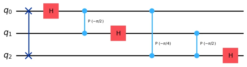
Since the state of the readout register needs to be arranged according to the order of this transformation, we don’t apply SWAP gate this time.

iqft = QFT(num_qubits=n_readout_qubits, inverse=True, do_swaps=True)
qc.append(iqft, [0, 1, 2])
qc.measure([0, 1, 2], [0, 1, 2])

When implementing the Quantum Fourier Transform and its inverse, it is important to pay close attention to the order in which operations are applied. In this case, by constructing the inverse Quantum Fourier Transform circuit while taking into account the pattern of controlled-$S$ gates applied to each qubit, we can obtain the expected result.

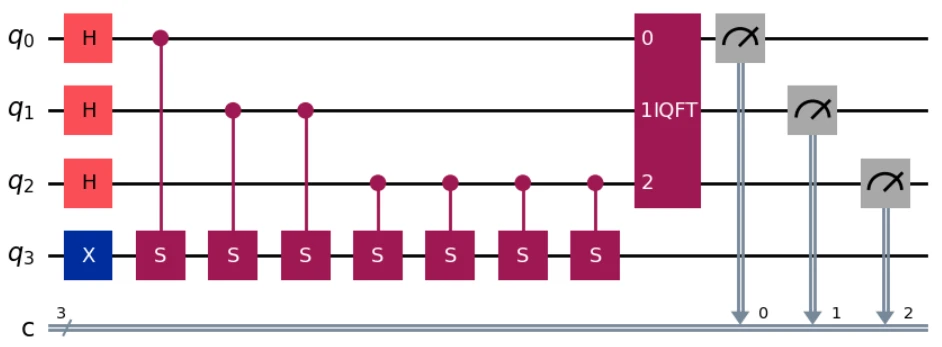
Printing the circuit by qc.draw('mpl') yields the following:

Now, let’s execute the quantum circuit.

pub = (qc, None)
job = sampler.run([pub], shots=1024)
result=job.result()[0]
print(result.data.c.get_counts())
# Output
# Counter({'010': 1024})

By measuring only the readout register, we obtain 010. Since the number of qubits in the readout register was $3$, this means that $\phi = 2/2^3 = 1/4$ was estimated by this circuit.

In other words, the eigenvalue of the $S$ gate with respect to $\ket{1}$ is estimated as $e^{2\pi i \phi} = e^{\pi i /2}$. This is indeed consistent with the theoretical expression below.
Quantum phase estimation has been successfully executed!

$$ S |1\rangle = \begin{bmatrix} 1 & 0 \\ 0 & e^{i\pi/2} \end{bmatrix} \begin{bmatrix} 0 \\ 1 \end{bmatrix} = e^{i\pi/2} |1\rangle $$