IBM Quantum Developer Certification v2.X Sample Test Explanation Part 1

In 2025, a new certification aligned with the latest Qiskit version, “IBM Certified Quantum Computation using Qiskit v2.X Developer - Associate”, has been released.

By obtaining this certification, you can demonstrate your knowledge of Qiskit and quantum programming!

To earn this certification, you need to pass the exam titled “Exam C1000-179: Fundamentals of Quantum Computing Using Qiskit v2.X Developer” as mentioned in the URL above. IBM also provides a Sample Test related to this exam, which is available in the “Sample Test” section on the website linked above.
However, the explanations are not provided in the Sample Test page, so I will include clear explanations as much as possible. This page contains explanations for questions 1 to 10. For the explanations of questions 11 to 21, please refer to this page.

Amazon Braket Learning Course

I have also created a learning course on Amazon Braket, AWS’s quantum computing service.

Quantum Computing on AWS for Beginners: Amazon Braket

This course is designed for those with no prior knowledge of quantum computing or AWS, and by the end, you’ll even be able to learn about quantum machine learning. Take advantage of this opportunity to build your skills in quantum technologies!

Sample Test 1:

Which one of the following code fragments will generate the given output?

[[ 1.+0.j  0.+0.j  0.+0.j  0.+0.j]
 [ 0.+0.j -1.+0.j  0.+0.j  0.+0.j] 
 [ 0.+0.j  0.+0.j  1.+0.j  0.+0.j] 
 [ 0.+0.j  0.+0.j  0.+0.j -1.+0.j]] 

Options:

• A.

p = Pauli('IZ') 
print(p.to_matrix())

• B.

p = Pauli('-II') 
print(p.to_matrix())

• C.

p = Pauli('-ZI') 
print(p.to_matrix()) 

• D.

p = Pauli('ZZ') 
print(p.to_matrix()) 

Answer: A

Explanation: The Pauli() class appearing in the code is used to represent operators. In the Options, expressions like Pauli('IZ') represent the tensor product of Pauli matrices, such as $I \otimes Z$. The calculation of the tensor product of matrices can be expressed as follows:

$$ \begin{align*} X \otimes Y = \begin{pmatrix} X_{11} Y & X_{12} Y \\ X_{21} Y & X_{22} Y \end{pmatrix} &= \begin{pmatrix} X_{11} Y_{11} & X_{11} Y_{12} & X_{12} Y_{11} & X_{12} Y_{12} \\ X_{11} Y_{21} & X_{11} Y_{22} & X_{12} Y_{21} & X_{12} Y_{22} \\ X_{21} Y_{11} & X_{21} Y_{12} & X_{22} Y_{11} & X_{22} Y_{12} \\ X_{21} Y_{21} & X_{21} Y_{22} & X_{22} Y_{21} & X_{22} Y_{22} \end{pmatrix} \end{align*} $$

Here, $X$ and $Y$ are defined as follows:

$$ X = \begin{pmatrix} X_{11} & X_{12} \\ X_{21} & X_{22} \end{pmatrix}, \quad Y = \begin{pmatrix} Y_{11} & Y_{12} \\ Y_{21} & Y_{22} \end{pmatrix} $$ 　　

Furthermore, the gates $I$ and $Z$ that appear in the code are defined as follows:

$$ I = \begin{pmatrix} 1 & 0 \\ 0 & 1 \end{pmatrix}, \quad Z = \begin{pmatrix} 1 & 0 \\ 0 & -1 \end{pmatrix} $$ By taking these into account, let’s compute the matrices corresponding to each Option.
Option A represents $I \otimes Z$, and the calculation yields the following: $$ I \otimes Z = \begin{pmatrix} 1 & 0 & 0 & 0 \\ 0 & -1 & 0 & 0 \\ 0 & 0 & 1 & 0 \\ 0 & 0 & 0 & -1 \end{pmatrix} $$ This matches the matrix shown in the sample test, so option A is the correct answer.
The remaining options can be calculated as follows, and you can confirm that they do not match the matrix shown in the sample test.
As for B, it represents $-I \otimes I$, and the following result is obtained: $$ -I \otimes I = \begin{pmatrix} -1 & 0 & 0 & 0 \\ 0 & -1 & 0 & 0 \\ 0 & 0 & -1 & 0 \\ 0 & 0 & 0 & -1 \end{pmatrix} $$
As for C, it represents $-Z \otimes I$, and the following result is obtained: $$ -Z \otimes I = \begin{pmatrix} -1 & 0 & 0 & 0 \\ 0 & -1 & 0 & 0 \\ 0 & 0 & 1 & 0 \\ 0 & 0 & 0 & 1 \end{pmatrix} $$
As for D, it represents $Z \otimes Z$, and the following result is obtained: $$ Z \otimes Z = \begin{pmatrix} 1 & 0 & 0 & 0 \\ 0 & -1 & 0 & 0 \\ 0 & 0 & -1 & 0 \\ 0 & 0 & 0 & 1 \end{pmatrix} $$
　　
　　
　　

Sample Test 2:

Applying the Qiskit T Gate to a qubit in state |1> introduces which global phase?

Options:

• A. $\pi/2$ phase

• B. $- \pi/2$ phase 　　

• C. $- \pi/4$ phase

• D. $\pi/4$ phase

Answer: D

Explanation: There are several gates that perform rotations around the Z-axis, such as the T, S, and Z gates. These gates rotate the state $|1\rangle$ by a phase of $\pi/4$, $\pi/2$, and $\pi$, respectively. Therefore, the correct answer is D. 　　
　　
　　

Sample Test 3:

Given the following code fragment, what is the approximate probability that a measurement would result in a bit value of 1?

from qiskit import QuantumCircuit 
import numpy as np 
qc = QuantumCircuit(1) 
qc.reset(0) 
qc.ry(np.pi / 2, 0) 
qc.measure_all() 

Options:

• A. 0.8536
• B. 1.0
• C. 0.1464
• D. 0.5

Answer: D

Explanation: In the Sample Test code, QuantumCircuit(1) is used to define a single qubit. At this point, the qubit is in the $|0\rangle$ state, meaning that no matter how many times it is measured, the outcome will always be $|0\rangle$. In this state, the angle $\theta$, which represents the tilt from the Z-axis, is $0$.

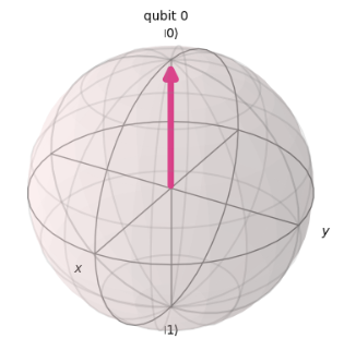
After this, qc.reset(0) is applied, which resets the 0th qubit to the $|0\rangle$ state. Since the qubit is already in the $|0\rangle$ state, this operation does not cause any change. Then, at the line qc.ry(np.pi / 2, 0), a rotation of the qubit around the Y-axis by an angle of $θ = \pi / 2$ is performed. After this operation, the qubit will be in the following state:

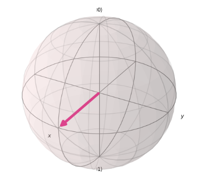
In this way, on the Bloch sphere, the vector tilts toward the direction of $|0>$ or $|1>$ depending on the value of $\theta$. When the tilt toward the $|0>$ direction is significant (i.e., $\theta < \pi/2$), the probability of measuring $|0>$ increases while the probability of measuring $|1>$ decreases. Conversely, when the tilt toward the $|1>$ direction is significant (i.e., $\pi/2 < \theta$), the probability of measuring $|1>$ increases while the probability of measuring $|0>$ decreases.
In this case, as shown in the diagram, the qubit points exactly halfway between $|0\rangle$ and $|1\rangle$, so the probabilities of measuring $|0\rangle$ and $|1\rangle$ are both $1/2$. Therefore, the correct answer is D.

Sample Test 4:

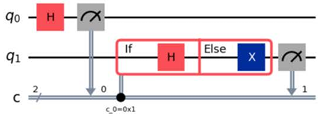
Which one of the following images is the output from the code below:

from qiskit import * 
qubits = QuantumRegister(2) 
clbits = ClassicalRegister(2) 
circuit = QuantumCircuit(qubits, clbits) 
(q0, q1) = qubits 
(c0, c1) = clbits 
circuit.h(q0) 
circuit.measure(q0, c0) 
with circuit.if_test((c0, 1)) as else_: 
    circuit.h(q1) 
with else_: 
    circuit.x(q1) 
circuit.measure(q1, c1) 

circuit.draw(output="mpl") 

Options:

• A.

  

• B.

  

• C.

  

• D.

  

Answer: A

Explanation: First, let’s look at the code for Sample Test.

from qiskit import * 
qubits = QuantumRegister(2) 
clbits = ClassicalRegister(2) 
circuit = QuantumCircuit(qubits, clbits) 
(q0, q1) = qubits 
(c0, c1) = clbits 

In the above code, the quantum bits $q0$ and $q1$, as well as the classical bits $c0$ and $c1$, are defined.

circuit.h(q0) 
circuit.measure(q0, c0) 

Next, in the above code, a Hadamard gate is applied to $q0$, and the result is measured and stored in $c0$.

with circuit.if_test((c0, 1)) as else_: 
    circuit.h(q1) 
with else_: 
    circuit.x(q1) 
circuit.measure(q1, c1) 

Then, a conditional branching operation is performed based on the measured value of $c0$. This means that if $c0$ is 1, a Hadamard gate is applied to $q1$; otherwise, an X gate is applied to $q1$.

circuit.draw(output="mpl") 

The final circuit is displayed here.
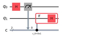
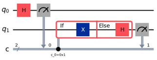
With these in mind, let’s look at the options. First, we can see that option B, which does not have an Else, is incorrect.
We can also see that option C, which applies an X gate in the if, is incorrect.
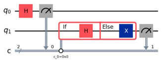
The only options remaining are options A and D, which differ in the formula at the bottom of the diagram. A has c_0=0x1 and D has c_0=0x0.
0x1 represents 1 in hexadecimal and 0x0 represents 0 in hexadecimal.

with circuit.if_test((c0, 1)) as else_: 

The above condition is written in the Sample Test, so A is the correct answer.

Sample Test 5:

Given the code fragment below, which image is the expected output?:

from qiskit.quantum_info import Statevector 
from qiskit.visualization import plot_histogram 
state = Statevector([0.+0.j, 0.+0.j, 0.70710678+0.j, 0.+0.j, 0.+0.j, -0.70710678+0.j, 0.+0.j, 0.+0.j]) 
counts = state.sample_counts(shots=1024) 
plot_histogram(counts)  

Options:

• A.

  

• B.

  

• C.

  

• D.

  

Answer: C

Explanation:

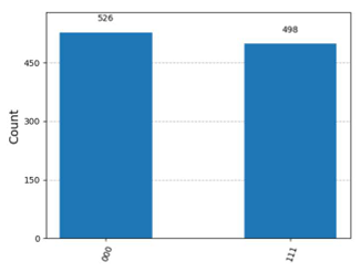
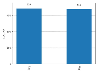
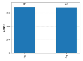
state = Statevector([0.+0.j, 0.+0.j, 0.70710678+0.j, 0.+0.j, 0.+0.j, -0.70710678+0.j, 0.+0.j, 0.+0.j]) 

The above code is included in the Sample Test, and since the vector has $8 = 2^3$ elements, we can see that the Statevector() represents the state of 3 qubits. Each element corresponds to the amplitude of the basis states in the following order: $|000\rangle$, $|001\rangle$, $|010\rangle$, $|011\rangle$, $|100\rangle$, $|101\rangle$, $|110\rangle$, $|111\rangle$.
Taking this into account, we can see that the coefficients of $|010\rangle$ and $|101\rangle$ are $0.70710678+0.j$ and $-0.70710678+0.j$, respectively. The squared absolute values of these coefficients represent the measurement probabilities. Since their absolute values are the same, $|010\rangle$ and $|101\rangle$ will be observed with equal probability.
Since C is the only diagram that corresponds to this, C is the correct answer.

Sample Test 6:

Which one of the following code fragments will generate the given qsphere representation visualization?
Note: the circles on the qsphere are the same color.

Options:

• A.

qc = QuantumCircuit(2) 
qc.h(0) 
qc.z(0) 
qc.cx(0, 1) 
state = Statevector(qc) 
plot_state_qsphere(state) 

• B.

qc = QuantumCircuit(2) 
qc.h(0) 
qc.z(0) 
qc.x(1) 
qc.cx(0, 1) 
state = Statevector(qc) 
plot_state_qsphere(state)

• C.

qc = QuantumCircuit(2) 
qc.x(1) 
qc.h(0) 
qc.cx(0, 1) 
state = Statevector(qc) 
plot_state_qsphere(state)

• D.

qc = QuantumCircuit(2) 
qc.h(0) 
qc.cx(0, 1) 
state = Statevector(qc) 
plot_state_qsphere(state) 

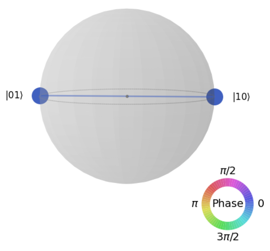
Answer: D

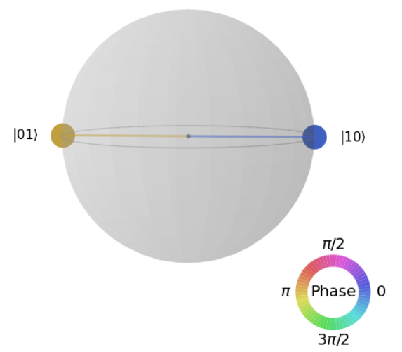
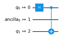
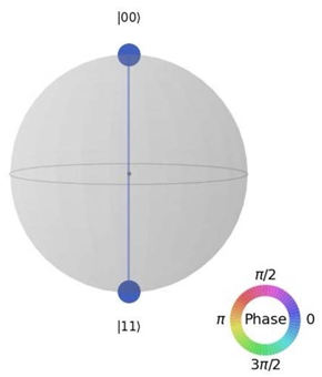
Explanation: In the diagram, the states $|00\rangle$ and $|11\rangle$ are shown, connected by the same blue color. In plot_state_qsphere(), when states are connected with the same color, it indicates that they share the same phase. This means that neither state has a coefficient like $e^{i \pi / 3}$ or a negative sign. This can be expressed mathematically as follows:

$$ \begin{align*} |\Phi^+\rangle &= \frac{1}{\sqrt{2}} (|00\rangle + |11\rangle) \\ \end{align*} $$

This state can be obtained as follows: starting from the initial state $|0\rangle \otimes |0\rangle$, apply an H gate to one of the qubits, and then apply a CX gate using using that qubit as the control.

$$ |0\rangle \otimes |0\rangle \xrightarrow{H_0} \frac{|0\rangle + |1\rangle}{\sqrt{2}} \otimes |0\rangle \xrightarrow{\text{CX}_{0,1}} \frac{|0\rangle \otimes |0\rangle + |1\rangle \otimes |1\rangle}{\sqrt{2}} $$ Since this rule is only applied in option D, the correct answer is D.
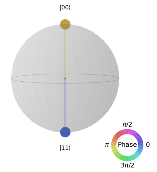
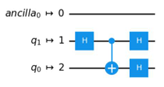
When you execute other options, different states will be displayed, as shown below.

For option A, compared to the correct answer D, an additional qc.z(0) is applied. qc.z(0) flips the phase of the $|1\rangle$ state. As a result, the state $\frac{1}{\sqrt{2}} (|00\rangle - |11\rangle)$ is realized, where the phase is inverted and combined. The corresponding diagram is shown below.

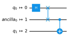
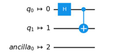
Sample Test 7:

Given the code fragment below, which of the following code fragments creates a rotation gate with an angle with an initially undefined value?

from qiskit.circuit import QuantumCircuit, Parameter, ParameterExpression 
qc = QuantumCircuit(1) 

Options:

• A.

theta = 3.14 
qc.rx(3.14, 0) 

• B.

theta = Parameter('theta') 
qc.rx(theta, 0) 

• C.

qc.rx('theta', 0)

• D.

qc.rx(ParameterExpression('theta'), 0) 

Answer: B

Explanation: In Qiskit, you can define quantum circuits with variables by using Parameter(). With this function, after defining the circuit, you can assign various values ​​to the variables and execute the quantum circuit. The correct way to use this function is option B, which is the correct answer.
The option A is incorrect because it fails to define the rotation gate using the angle as a variable.
C and D will result in an error when executed.

Sample Test 8:

Which one of the following types of register stores the result of a measured circuit?

Options:

• A. Ancilla register 　　

• B. Quantum register 　　

• C. Classical register 　　

• D. Circuit register 　　
  
  

Answer: C

Explanation: The explanation of Quantum register, Classical register, and Ancilla register can be found here. The Classical register in option C is used to store the measurement results after computation, and in this case, it is the correct answer.
The Ancilla register in option A is a register primarily used for error correction and algorithm implementation.
The Quantum register in opotion B is a register that holds quantum bits.
Circuit register in option D does not exist in qiskit.circuit.

Sample Test 9:

Given the code fragment below, which one of the following images could be produced?

from qiskit import QuantumCircuit 
from qiskit import generate_preset_pass_manager 
qc = QuantumCircuit(2) 
qc.h(0) 
qc.cx(0,1) 
pass_manager = generate_preset_pass_manager( 
    optimization_level=3, 
    coupling_map=[[0, 1], [1, 2]] , 
    basis_gates=['h', 'swap', 'cx'], 
    initial_layout=[0, 2] ) 
tqc = pass_manager.run(qc) 
tqc.draw(output="mpl")   

Options:

• A.

  

• B.

  

• C.

  

• D.

  

Answer: A

Explanation: Let’s take a look at the code first.

from qiskit import QuantumCircuit 
from qiskit import generate_preset_pass_manager 
qc = QuantumCircuit(2) 
qc.h(0) 
qc.cx(0,1) 

This code defines the quantum circuit that applies the H gate and the CX gate.

pass_manager = generate_preset_pass_manager( 
    optimization_level=3, 
    coupling_map=[[0, 1], [1, 2]] , 
    basis_gates=['h', 'swap', 'cx'], 
    initial_layout=[0, 2] ) 

generate_preset_pass_manager() is a function that transforms quantum circuits for use on real quantum computers or in environments with various constraints. Moreover, as shown in this code, even without specifying an actual quantum computer, you can define a virtual environment by setting different constraints yourself.
Let’s take a look at its arguments.

coupling_map=[[0, 1], [1, 2]] indicates that connections exist only between virtual physical qubits 0 and 1, and between the qubits 1 and 2. For example, this can be represented in a diagram as follows:

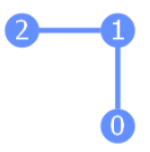
As shown here, there is no connection between the qubits 0 and 2. Therefore, it is not possible to apply a CX gate between qubits 0 and 2. This is an important point in this Sample Test. The setting basis_gates=['h', 'swap', 'cx'] defines the constraint that, in this virtual environment, only the H gate, Swap gate, and CX gate are supported.

The setting initial_layout=[0, 2] maps quantum bit q0 defined in qc to physical qubit 0, and quantum bit q1 to physical qubit 2 before computation begins. Some may wonder why such constraints are explicitly specified. In fact, when working with actual quantum hardware, such constraints are often present. Therefore, performing computations with these constraints in a local environment serves as a valuable method for validating behavior in anticipation of running on real quantum devices.

optimization_level=3 means how much optimization the pass_manager should do when converting quantum circuits for this environment, with 3 being the highest level.

tqc = pass_manager.run(qc) 
tqc.draw(output="mpl")  

In this part, the originally defined circuit qc is converted into a quantum circuit tqc that is tailored to the virtual environment using pass_manager, and the circuit is displayed.
Now, let’s take a look at the Options.
The option B is incorrect because it does not reflect the setting initial_layout=[0, 2], which maps qubit q0 onto physical qubit 0 and qubit q1 onto physical qubit 2.
The option C is incorrect because an undefined H gate has been inserted at the very end of the circuit.
The option D reflects the setting initial_layout=[0, 2], which maps qubit q0 to physical qubit 0 and qubit q1 to physical qubit 2 before computation. At first glance, this may seem correct. However, as previously explained, it is not possible to apply a CX gate directly between physical qubits 0 and 2 in this case. When such a constraint exists, generate_preset_pass_manager() automatically transforms the circuit into an executable form-like in OptionsA-by inserting Swap gates to exchange qubit positions. Therefore, D is incorrect and A is correct.

Sample Test 10:

Which three of the following are job execution modes in Qiskit Runtime?

Options:

• A. classical

• B. session

• C. parallel

• D. quantum

• E. batch

• F. single job

Answer: B, E, F

Explanation: The execution modes of Qiskit Runtime are described here. As described there, there are three execution modes for Qiskit Runtime: session, batch, and single job. Therefore, answers B, E, and F are correct. Each mode is explained below.
The single job mode is the simplest mode. It is convenient when you want to try running a single job.
The batch mode is useful for executing multiple jobs together. However, since they are treated as batch processing, it is important to note that there is no guarantee the jobs will be executed in the order they were submitted.
In session mode, a dedicated time slot is allocated during which the system can be used exclusively. In variational algorithms such as VQC and VQE, computations alternate between classical and quantum computers. If the system has to wait for other users’ jobs each time a quantum computation is performed, it can take a considerable amount of time. By using session mode, such delays are avoided, allowing variational algorithms to be executed much more efficiently.

For the explanations of questions 11 to 21, please refer to this page.

Amazon Braket Learning Course

I have also created a learning course on Amazon Braket, AWS’s quantum computing service.

Quantum Computing on AWS for Beginners: Amazon Braket

This course is designed for those with no prior knowledge of quantum computing or AWS, and by the end, you’ll even be able to learn about quantum machine learning. Take advantage of this opportunity to build your skills in quantum technologies!