Quantum Machine Learning on AWS Amazon Braket: QCBM
As described in another article, Amazon Braket, AWS’s quantum computing service, allows users to easily access various features through the Amazon Braket SDK, a software development kit for quantum computing. In this article, we explain how to run quantum machine learning algorithms—machine learning techniques that leverage quantum computers.
Amazon Braket Learning Course
You can efficiently learn the basic knowledge of quantum computing—including quantum gates and quantum circuits introduced in this article—as well as how to use Amazon Braket through this course.

This course is designed for those with no prior knowledge of quantum computing or AWS, and by the end, you’ll even be able to learn about quantum machine learning. Take advantage of this opportunity to build your skills in quantum technologies!
Quantum Machine Learning on AWS Amazon Braket: QCBM
Several approaches to quantum machine learning algorithms have been proposed, but in this article, we will focus on implementing the Quantum Circuit Born Machine (QCBM). This algorithm enables the construction of generative models through unsupervised learning and is already available in Amazon Braket’s algorithm library.
https://github.com/amazon-braket/amazon-braket-algorithm-library/tree/main/src/braket/experimental/algorithms/quantum_circuit_born_machine
In this article, we will use this library.
Environment Setup
If you’re using an Amazon Braket Notebook instance, no additional setup is required. However, if you’re working on your local machine or a server, you’ll need to install the Amazon Braket SDK and Jupyter Notebook. Additionally, to use the Amazon Braket Algorithm Library, we will run a few extra installation steps.
git clone https://github.com/amazon-braket/amazon-braket-algorithm-library.git
cd amazon-braket-algorithm-library
pip install .
The following steps are executed within a Jupyter Notebook environment.
Training Dataset Overview
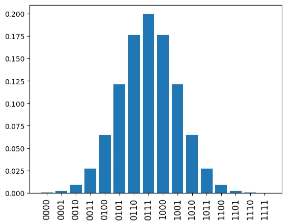
With 4 qubits, it is possible to represent $2^4$ different bitstrings. A Gaussian distribution with a peak near the center of these bitstrings can be generated as follows.
import numpy as np
n_qubits = 4
def gaussian(n_qubits, mu, sigma):
    x = np.arange(2**n_qubits)
    gaussian = 1.0 / np.sqrt(2 * np.pi * sigma**2) * np.exp(-((x - mu) ** 2) / (2 * sigma**2))
    return gaussian / sum(gaussian)

data = gaussian(n_qubits, mu=7, sigma=2)
data = data / sum(data)
The figure below shows a Gaussian distribution centered around the middle of the 4-qubit bitstrings. This distribution will be used as the training data in this example.
import matplotlib.pyplot as plt
%matplotlib inline
labels = [format(i, "b").zfill(n_qubits) for i in range(len(data))]
plt.bar(range(2**n_qubits), data)
plt.xticks(list(range(len(data))), labels, rotation="vertical", size=12)
plt.show()
Execution of Quantum Machine Learning Algorithm
We will import the necessary functions.
from braket.devices import LocalSimulator
from braket.experimental.algorithms.quantum_circuit_born_machine import QCBM, mmd_loss
In this case, we will use a local device since the computation will be performed locally. Running hybrid algorithms like QCBM on AWS Managed Simulators or quantum computers can lead to high costs. For circuits of this scale, a local simulator is sufficient for computation, so it’s best to take advantage of local simulators.
device = LocalSimulator()
Since the training data consists of 4-bit strings, we define the number of qubits accordingly as 4.
n_qubits = 4
In QCBM, similar to deep learning, you can define the number of layers. In this case, let’s set the number of layers to 4. With these parameters, you can create an instance of QCBM as follows.
n_layers = 4
qcbm = QCBM(device, n_qubits, n_layers, data)
Let’s draw the quantum circuit defined by this. There are four layers defined.
T  : │         0         │         1         │         2         │  3  │         4         │         5         │         6         │         7         │         8         │         9         │        10         │        11         │        12         │        13         │        14         │        15         │        16         │        17         │        18         │ 19  │ 20  │ Result Types  │
      ┌─────────────────┐ ┌─────────────────┐ ┌─────────────────┐       ┌─────────────────┐ ┌─────────────────┐ ┌─────────────────┐                                         ┌─────────────────┐ ┌─────────────────┐ ┌─────────────────┐                                         ┌─────────────────┐ ┌─────────────────┐ ┌─────────────────┐                                                     ┌─────────────┐
q0 : ─┤ Rx(theta_0_0_0) ├─┤ Rz(theta_0_0_1) ├─┤ Rx(theta_0_0_2) ├───●───┤ Rx(theta_1_0_0) ├─┤ Rz(theta_1_0_1) ├─┤ Rx(theta_1_0_2) ├──────────────────────────────●──────────┤ Rx(theta_2_0_0) ├─┤ Rz(theta_2_0_1) ├─┤ Rx(theta_2_0_2) ├──────────────────────────────●──────────┤ Rx(theta_3_0_0) ├─┤ Rz(theta_3_0_1) ├─┤ Rx(theta_3_0_2) ├──────────────────────────────●──────────────────────┤ Probability ├─
      └─────────────────┘ └─────────────────┘ └─────────────────┘   │   └─────────────────┘ └─────────────────┘ └─────────────────┘                              │          └─────────────────┘ └─────────────────┘ └─────────────────┘                              │          └─────────────────┘ └─────────────────┘ └─────────────────┘                              │                      └──────┬──────┘
      ┌─────────────────┐ ┌─────────────────┐ ┌─────────────────┐ ┌─┴─┐                     ┌─────────────────┐ ┌─────────────────┐ ┌─────────────────┐        ┌─┴─┐                            ┌─────────────────┐ ┌─────────────────┐ ┌─────────────────┐        ┌─┴─┐                            ┌─────────────────┐ ┌─────────────────┐ ┌─────────────────┐        ┌─┴─┐                    ┌──────┴──────┐
q1 : ─┤ Rx(theta_0_1_0) ├─┤ Rz(theta_0_1_1) ├─┤ Rx(theta_0_1_2) ├─┤ X ├──────────●──────────┤ Rx(theta_1_1_0) ├─┤ Rz(theta_1_1_1) ├─┤ Rx(theta_1_1_2) ├────────┤ X ├─────────────────●──────────┤ Rx(theta_2_1_0) ├─┤ Rz(theta_2_1_1) ├─┤ Rx(theta_2_1_2) ├────────┤ X ├─────────────────●──────────┤ Rx(theta_3_1_0) ├─┤ Rz(theta_3_1_1) ├─┤ Rx(theta_3_1_2) ├────────┤ X ├──────────●─────────┤ Probability ├─
      └─────────────────┘ └─────────────────┘ └─────────────────┘ └───┘          │          └─────────────────┘ └─────────────────┘ └─────────────────┘        └───┘                 │          └─────────────────┘ └─────────────────┘ └─────────────────┘        └───┘                 │          └─────────────────┘ └─────────────────┘ └─────────────────┘        └───┘          │         └──────┬──────┘
      ┌─────────────────┐ ┌─────────────────┐ ┌─────────────────┐              ┌─┴─┐                            ┌─────────────────┐ ┌─────────────────┐ ┌─────────────────┐        ┌─┴─┐                            ┌─────────────────┐ ┌─────────────────┐ ┌─────────────────┐        ┌─┴─┐                            ┌─────────────────┐ ┌─────────────────┐ ┌─────────────────┐ ┌─┴─┐       ┌──────┴──────┐
q2 : ─┤ Rx(theta_0_2_0) ├─┤ Rz(theta_0_2_1) ├─┤ Rx(theta_0_2_2) ├──────────────┤ X ├─────────────────●──────────┤ Rx(theta_1_2_0) ├─┤ Rz(theta_1_2_1) ├─┤ Rx(theta_1_2_2) ├────────┤ X ├─────────────────●──────────┤ Rx(theta_2_2_0) ├─┤ Rz(theta_2_2_1) ├─┤ Rx(theta_2_2_2) ├────────┤ X ├─────────────────●──────────┤ Rx(theta_3_2_0) ├─┤ Rz(theta_3_2_1) ├─┤ Rx(theta_3_2_2) ├─┤ X ├───●───┤ Probability ├─
      └─────────────────┘ └─────────────────┘ └─────────────────┘              └───┘                 │          └─────────────────┘ └─────────────────┘ └─────────────────┘        └───┘                 │          └─────────────────┘ └─────────────────┘ └─────────────────┘        └───┘                 │          └─────────────────┘ └─────────────────┘ └─────────────────┘ └───┘   │   └──────┬──────┘
      ┌─────────────────┐ ┌─────────────────┐ ┌─────────────────┐                                  ┌─┴─┐        ┌─────────────────┐ ┌─────────────────┐ ┌─────────────────┐                            ┌─┴─┐        ┌─────────────────┐ ┌─────────────────┐ ┌─────────────────┐                            ┌─┴─┐        ┌─────────────────┐ ┌─────────────────┐ ┌─────────────────┐       ┌─┴─┐ ┌──────┴──────┐
q3 : ─┤ Rx(theta_0_3_0) ├─┤ Rz(theta_0_3_1) ├─┤ Rx(theta_0_3_2) ├──────────────────────────────────┤ X ├────────┤ Rx(theta_1_3_0) ├─┤ Rz(theta_1_3_1) ├─┤ Rx(theta_1_3_2) ├────────────────────────────┤ X ├────────┤ Rx(theta_2_3_0) ├─┤ Rz(theta_2_3_1) ├─┤ Rx(theta_2_3_2) ├────────────────────────────┤ X ├────────┤ Rx(theta_3_3_0) ├─┤ Rz(theta_3_3_1) ├─┤ Rx(theta_3_3_2) ├───────┤ X ├─┤ Probability ├─
      └─────────────────┘ └─────────────────┘ └─────────────────┘                                  └───┘        └─────────────────┘ └─────────────────┘ └─────────────────┘                            └───┘        └─────────────────┘ └─────────────────┘ └─────────────────┘                            └───┘        └─────────────────┘ └─────────────────┘ └─────────────────┘       └───┘ └─────────────┘
T  : │         0         │         1         │         2         │  3  │         4         │         5         │         6         │         7         │         8         │         9         │        10         │        11         │        12         │        13         │        14         │        15         │        16         │        17         │        18         │ 19  │ 20  │ Result Types  │

Unassigned parameters: [theta_0_0_0, theta_0_0_1, theta_0_0_2, theta_0_1_0, theta_0_1_1, theta_0_1_2, theta_0_2_0, theta_0_2_1, theta_0_2_2, theta_0_3_0, theta_0_3_1, theta_0_3_2, theta_1_0_0, theta_1_0_1, theta_1_0_2, theta_1_1_0, theta_1_1_1, theta_1_1_2, theta_1_2_0, theta_1_2_1, theta_1_2_2, theta_1_3_0, theta_1_3_1, theta_1_3_2, theta_2_0_0, theta_2_0_1, theta_2_0_2, theta_2_1_0, theta_2_1_1, theta_2_1_2, theta_2_2_0, theta_2_2_1, theta_2_2_2, theta_2_3_0, theta_2_3_1, theta_2_3_2, theta_3_0_0, theta_3_0_1, theta_3_0_2, theta_3_1_0, theta_3_1_1, theta_3_1_2, theta_3_2_0, theta_3_2_1, theta_3_2_2, theta_3_3_0, theta_3_3_1, theta_3_3_2].
Also, let’s set the number of training iterations to 10.
n_iterations = 10
As the number of gates in this circuit indicates, we need 3 * n_layers * n_qubits parameters this time.
Now, let’s define the initial values for these parameters.
init_params = np.random.rand(3 * n_layers * n_qubits) * np.pi * 2
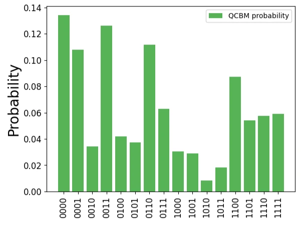
Using qcbm.get_probabilities(init_params), we can obtain the probability distribution from the circuit in this initial state.
Since no training has been done yet, it can be confirmed that the output probability distribution is completely different from the target data, as shown below.
qcbm_probs = qcbm.get_probabilities(init_params)

plt.bar(range(2**n_qubits), qcbm_probs, label="QCBM probability", alpha=0.8, color="tab:green")
plt.xticks(list(range(len(data))), labels, rotation="vertical", size=12)
plt.yticks(size=12)
plt.ylabel("Probability", size=20)

plt.legend()
plt.show()
Now, let’s proceed with training the model.
The gradients are computed using qcbm.gradient(x).
From the code, it appears that the gradient calculation follows the method described in this paper.
The loss function used is Maximum Mean Discrepancy (MMD) Loss.
Therefore, the training is carried out using scipy as shown below.
from scipy.optimize import minimize

history = []

def callback(x):
    loss = mmd_loss(qcbm.get_probabilities(x), data)
    history.append(loss)

result = minimize(
    lambda x: mmd_loss(qcbm.get_probabilities(x), data),
    x0=init_params,
    method="L-BFGS-B",
    jac=lambda x: qcbm.gradient(x),
    options={"maxiter": n_iterations},
    callback=callback,
)
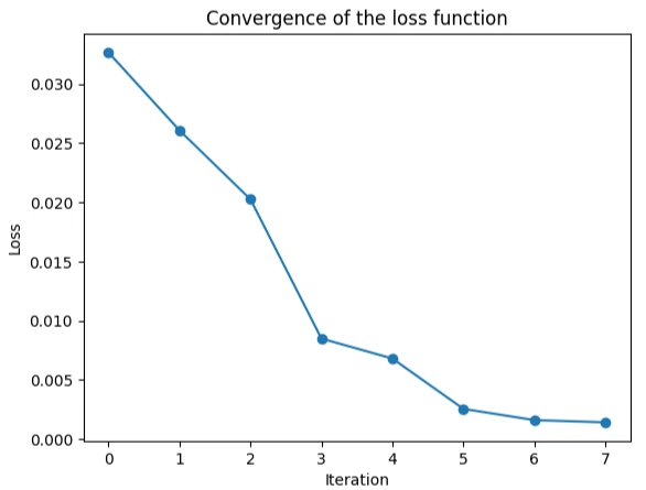
The convergence of the loss function during training is shown below.
plt.plot(history, "-o")
plt.xlabel("Iteration")
plt.ylabel("Loss")
plt.title("Convergence of the loss function")
Now, let’s use the parameters after training to obtain the probability distribution and compare it with the target data.
qcbm_probs = qcbm.get_probabilities(result["x"])

plt.bar(range(2**n_qubits), data, label="target probability", alpha=1, color="tab:blue")
plt.bar(range(2**n_qubits), qcbm_probs, label="QCBM probability", alpha=0.8, color="tab:green")
plt.xticks(list(range(len(data))), labels, rotation="vertical", size=12)
plt.yticks(size=12)

plt.xlabel("Sample", size=20)
plt.ylabel("Probability", size=20)

plt.legend()
plt.show()
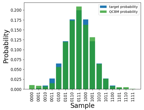
It has been confirmed that training has progressed from the initial parameter values.
Amazon Braket Learning Course
You can efficiently learn the basic knowledge of quantum computing—including quantum gates and quantum circuits introduced in this article—as well as how to use Amazon Braket through this course.
This course is designed for those with no prior knowledge of quantum computing or AWS, and by the end, you’ll even be able to learn about quantum machine learning. Take advantage of this opportunity to build your skills in quantum technologies!