Shor's Algorithm with AWS Amazon Braket

In the previous articles, we covered the following topics:

Based on this, we will study Shor’s algorithm, a quantum algorithm said to be capable of breaking RSA encryption and ECDSA encryption used in Bitcoin transactions.

Amazon Braket Learning Course

You can efficiently learn the basic knowledge of quantum computing—including quantum gates and quantum circuits introduced in this article—as well as how to use Amazon Braket through this course.

https://www.udemy.com/course/quantum-computing-on-aws-for-beginners-amazon-braket/?referralCode=F361C3FD774489A1B5B8

This course is designed for those with no prior knowledge of quantum computing or AWS, and by the end, you’ll even be able to learn about quantum machine learning. Take advantage of this opportunity to build your skills in quantum technologies!

Regarding the IBM Quantum Developer Certification Exam

IBM offers a certification exam related to Qiskit, which is introduced in this blog.

By obtaining this certification, you can prove your knowledge of Qiskit and quantum programming. For those aiming to achieve this certification, I have created a practice exams on the Udemy platform! I have made the explanations as clear as possible, so please make sure to take full advantage of the following practice exams as extra study material for exam preparation.

Practice exams

https://www.udemy.com/course/ibm-certified-quantum-computation-qiskit-practice-exams/?referralCode=3B3263DF800E05439AD2

Shor’s algorithm

If quantum computers become capable of handling a sufficient number of qubits, it is said that Shor’s algorithm could pose a threat to RSA and ECDSA encryption. For example, RSA encryption is based on the difficulty of factoring large integers. In this section, we will look at how Shor’s algorithm can be used to factor such integers. The process of factoring an integer $N$ using this algorithm is as follows:

Choose an $a$ such that $1 < a < N$ and the greatest common divisor of $a$ and $N$ is $1$.
　　　　　$\downarrow$
Determine the period $r$ of the function $a^x \bmod\ N$.
　　　　　$\downarrow$
Find a factor of $N$ by computing the greatest common divisor of $a^{\frac{r}{2}} \pm 1$ and $N$.

Here, it mentions ‘Determine the period $r$ of the function $a^x \bmod\ N$,’ so let’s look at a concrete example.

As an example, let’s consider factoring $N = 39$ by choosing $a = 5$. The graph of $a^x \bmod\ N = 5^x \bmod\ 39$, with $x$ on the horizontal axis, is shown below.

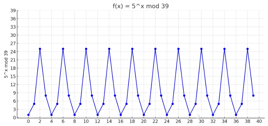
Listing the values on the y-axis, we can see that this is a periodic function that returns to its original value after four changes.

$$ 1 \rightarrow 5 \rightarrow 25 \rightarrow 8 \rightarrow 1 \rightarrow 5 \rightarrow 25 \rightarrow 8 \tag{1} $$

This period corresponds to the order $r$, and since the function returns to its original value after 4 steps in this case, we find that $r = 4$. Shor’s algorithm leverages a quantum computer to efficiently compute this $r$, enabling fast factorization.

When it comes to implementing Shor’s algorithm, there are two main approaches. One is a general-purpose but complex method that directly defines and uses the function $a^x \bmod\ N$ within a quantum circuit, as described in this paper. The other is a simpler implementation that defines and uses an operator based on the observed behavior of $a^x \bmod\ N$ for specific pairs of $a$ and $N$.

In this explanation, we will focus on the simpler implementation method tailored to a specific pair of $a$ and $N$.

To begin, let’s go through the initial setup. The operator that produces the periodic behavior of the function $a^x \bmod\ N$ can be expressed as follows.

$$ U |y\rangle = |a y\bmod\ N\rangle \tag{2} $$

Let’s look at an example to better understand this. We’ll consider the case we’ve already seen, where $N = 39$ and $a = 5$. In this case, the expression is as follows.

$$ U |y\rangle = |5 y\bmod\ 39\rangle $$

When substituting $y = 1$, we obtain the following result.

$$ U |1\rangle = |5 \cdot 1\bmod\ 39\rangle = |5\rangle $$

Substituting this result back into $y$, we obtain the following.

$$ U |5\rangle = |5 \cdot 5\bmod\ 39\rangle = |25\rangle $$

Let’s substitute this result once again.

$$ U |25\rangle = |5 \cdot 25\bmod\ 39\rangle = |8\rangle $$

We substitute it again.

$$ U |8\rangle = |5 \cdot 8\bmod\ 39\rangle = |1\rangle $$

The result has returned to $1$! Indeed, this operator successfully reproduces the transformation described in (1), and it gives us hope that we might be able to determine the order $r$ using this operator. (Of course, we may already know the value of $r$ at this point, but since the goal is to derive the answer from the quantum circuit, we’ll pretend we don’t.)

Here, it is known that the eigenvalues of $U$ satisfying condition (2), with eigenstates denoted as $|u_s\rangle$, are given as follows.

$$ U|u_s\rangle =\ e^{\frac{2\pi i s}{r}}|u_s\rangle $$

This is a form that allows us to derive the solution using the Quantum Phase Estimation algorithm! Furthermore, the eigenstates of this operator can be expressed as follows.

$$ |u_s\rangle = \frac{1}{\sqrt{r}} \sum_{k=0}^{r-1} e^{-\frac{2\pi i s k}{r}}
\bigl|a^{k}\bmod N\bigr\rangle \quad (s = 0,1,\dots,r-1) $$

These eigenstates have a special property: when summed over all $s$, the result is $|1\rangle$.

$$ |1\rangle = \frac{1}{\sqrt{r}} ( |u_0\rangle + |u_1\rangle +….. |u_{r-1}\rangle ) $$

In the Quantum Phase Estimation algorithm, we can determine the eigenvalue corresponding to a given eigenstate by defining that eigenstate using qubits. Based on this property, by setting the eigenstate-defining qubit to $|1\rangle$ and executing quantum phase estimation, we obtain a superposition of eigenvalues $|\psi\rangle$ as shown below. Here, $n$ denotes the number of qubits in the readout register.

$$ |\psi\rangle = \frac{1}{\sqrt{r}} ( |2^n\cdot\frac{0}{r}\rangle + |2^n\cdot\frac{1}{r}\rangle +… + |2^n\cdot\frac{r - 1}{r}\rangle ) $$

Since the information about $r$ is embedded in this state, by measuring $|\psi\rangle$, we can estimate the value of $r$ from the result. The overall procedure of this method can be summarized as follows:

Define the operator $U$ such that, for the given $a$ and $N$, it transforms the state as $U |y\rangle = |a y \bmod\ N\rangle$.
　　　　　$\downarrow$
Perform quantum phase estimation on the operator $U$ using the superposition of eigenstates $|1\rangle$.
　　　　　$\downarrow$
Estimate $r$ from the measurement result.

Let’s try it out!

Shor’s algorithm with Amazon Braket SDK

Let’s take this opportunity to try factoring a larger number, $N = 341$. We’ll set $a = 32$ for this implementation. First, we define the operator $U$ such that $U |y\rangle = |a y \bmod\ N\rangle$ for $a = 32$ and $N = 341$. By substituting $y = 1$, we obtain the following result. $$ U |1\rangle = |32 \cdot 1\bmod\ 341\rangle = |32\rangle $$ Let’s substitute this result once again. $$ U |32\rangle = |32 \cdot 32\bmod\ 341\rangle = |1\rangle $$ The state has returned to $|1\rangle$! Therefore, the transformation can be described as follows.

$$ |1\rangle \rightarrow |32\rangle \rightarrow |1\rangle \rightarrow |32\rangle \rightarrow |1\rangle \tag{3} $$ This transformation by $U$ can be implemented by applying an X gate to the 6th qubit of the eigenstate register. Now, let’s perform the Quantum Phase Estimation algorithm using this $U$ and the state $|1\rangle$. To begin, we will follow the code introduced in this article, starting with applying Hadamard gates to the readout register.

from braket.circuits import Circuit
from braket.devices import LocalSimulator
from braket.experimental.algorithms.quantum_fourier_transform import (
    quantum_fourier_transform as qft_module
)

n_readout_qubits = 3
circ = Circuit()

for qubit in list(range(n_readout_qubits)):
    circ.h(qubit)

We will now define $|1\rangle$ as follows.

circ.x(n_readout_qubits)

Then, we apply the controlled-$U$ gate that induces the change in (3), following the rules of the quantum phase estimation algorithm.

n_eigenstate_qubits = 6
for ctl_bit in list(range(n_readout_qubits)):
    for i in list(range(2**(ctl_bit))):
        circ.cnot(ctl_bit, n_readout_qubits + n_eigenstate_qubits - 1)

Finally, We apply inverse Quantum Fourier Transformation.

circ.swap(0,n_readout_qubits - 1)
circ.iqft(range(n_readout_qubits))
circ.measure([0, 1, 2])
device = LocalSimulator()
result = device.run(circ, shots=1000).result()
counts = result.measurement_counts
print(counts)
# Output
# Counter({'000': 501, '100': 499})

For code that estimates $r$ from such results, please refer to this get_factors_from_results() function. In this case, we can estimate $r = 2$ from the results. Using this value of $r$, we obtain $a^{\frac{r}{2}} + 1 = 33$ and $a^{\frac{r}{2}} - 1 = 31$. The greatest common divisors of these two numbers with 341 are as follows.

$$ \begin{align} gcd(33, 341) = 11 \\ gcd(31, 341) = 31 \end{align} $$ We have successfully found the prime factors of 341: 11 and 31!